

Java remains one of the most widely used programming languages today, especially in enterprise backend systems—and for many good reasons. With each new release, Java’s robust runtime offers additional improvements in performance, security, scalability, and developer productivity. The portability of its code has proven increasingly relevant and useful as the industry embraces ARM64, making Java one of the go-to languages for modern workloads. And Java’s rich ecosystem of libraries provides developers with prebuilt, reliable solutions for a wide range of functions—including web development, data processing, security, and machine learning. At Datadog, we too use Java for a wide range of workloads in our own cloud infrastructure—and contribute back to the ecosystem.
However, because Java was designed before the ubiquity of cloud computing, developers face specific challenges when running their Java applications on Kubernetes and other container orchestrators, particularly when using older frameworks such as Spring. For starters, Java often has higher memory and CPU requirements than natively compiled languages such as Rust, owing to the overhead of both the Java Virtual Machine (JVM) and Garbage Collection (GC). Additionally, older frameworks and libraries in the Java ecosystem can significantly increase startup times. This problem is especially common in container orchestration environments such as Kubernetes, where pods are ephemeral. All the added startup time that comes from spinning up new containers can be a drag on the scaling-up process.
While you can often allocate more resources to improve performance—increasing the amount of CPU and RAM allocated to your Java pods—a poorly tuned application is an unnecessary cost sink. There are a number of ways to tune your Java applications beyond simply adding resources, which we will explore here. In this post, we’ll explain:
- How the JVM works
- How to select versions of the JVM, frameworks, and server software
- How to tune Kubernetes deployments of Java applications
- How to tune the JVM for ephemeral, container-based infrastructure
- How to configure Java Garbage Collection for a containerized environment
- How to improve JVM startup times
- How to monitor Java applications with Datadog
How the JVM works
The JVM is an evolving, platform-independent runtime environment that enables Java applications to run consistently. Before an application is launched, the Java Development Kit (JDK) compiles code to bytecode—an intermediate, interoperable version of the source code—which gives Java its portability. When the JVM launches an application and encounters a Java function in the bytecode for the first time, it interprets it—translating and executing each bytecode instruction sequentially.
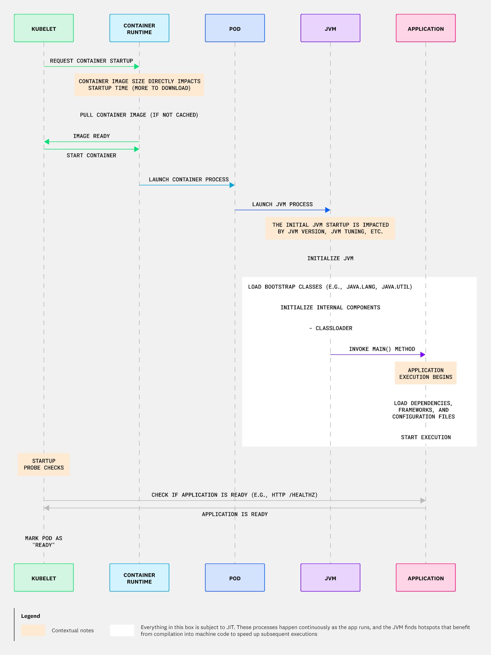
As the JVM continues to run, the Just-In-Time (JIT) compiler in the JVM monitors method execution frequencies and identifies hotspots (frequently executed code sections). The JIT compiler may decide to compile these hotspots into native machine code, speeding up subsequent executions. Additionally, in most modern JVM implementations, tiered compilation is enabled by default. This means that for semi-frequently executed functions, it will use the C1 compiler, a relatively fast compiler that improves execution times compared to bytecode. For very frequently executed operations, it compiles code with the C2 compiler, which provides the best runtime performance of the resultant code. However, C2 compilation requires more compilation time and is thus reserved only for the hottest of hotspots. Through its use of the C1 and C2 compiler, the JVM here thus makes tradeoffs between compilation time and runtime performance. For a visual illustration of how this works in Kubernetes, see the diagram below.
The relative complexity and rich functionality of the JVM can lead to long startup times. Consequently, a common goal when tuning the JVM in modern environments like Kubernetes or cloud-hosted serverless (which is effectively a containerized environment with very fast startup speed expectations) is to minimize the time-to-start for the JVM. Once the JVM is started, we also want to start executing main() as quickly as possible. But to achieve this goal, it’s important to understand the tradeoffs between running interpreted bytecode vs. JIT-compiled code. We cover this topic in detail later in this blog post.
Select versions of the JVM, frameworks, and server software to optimize performance
A common cause of sluggish startup times is the use of older frameworks (e.g., Spring Boot, EJB), outdated JDKs, or complex application servers (e.g., Weblogic). Because different software components lead to noticeable differences in application performance, engineers should thoroughly research tech choices to assess their impact on JVM initialization. For example, if you have an older, EJB3 application running on Weblogic that you’d like to host on Kubernetes, it would be advisable to transition to a more modern framework if possible. However, switching frameworks could admittedly be impractical in some scenarios.
Slow startup times can also result from maintenance issues as simple as not using the latest JVM, as huge strides have been and continue to be made in improving the JVM’s performance. (If you’d like to learn more about the performance and security enhancements associated with Java versions, check out this Oracle blog post.)
Next, some OpenJDK distributions are more performance-oriented than others, and in some cases, exploring alternatives might be worthwhile. There are a plethora of distributions of the OpenJDK, which include vendor-specific optimizations and tools for the Java platform. For example, Coretto is Amazon’s distribution of the OpenJDK, and Azul’s Platform Prime is a performance-optimized solution that is valuable for organizations with latency-sensitive, large-scale, or resource-intensive workloads.
Another interesting technology that can improve performance is GraalVM. GraalVM is an advanced JDK that offers an AOT tool, native-image, which compiles Java code into native machine code before runtime. This essentially turns Java into a compiled language like C++ or golang and eliminates the need for JIT compilation. For simplicity, Quarkus enables you to use Graal out of the box, making it easier to implement and helping reduce the risk of error that can otherwise be a drawback to using Graal. To illustrate this ease of use, you can build a native image using Quarkus and Graal with this simple command: quarkus build --native.
All these options mentioned above can improve startup times as well as offer significant memory usage improvements compared to what is typical for traditional JVM execution.
How to tune a Kubernetes deployment running a Java application
To help ensure that your Java applications run efficiently, it’s crucial to tune your Kubernetes infrastructure with this purpose in mind.
Allocate adequate resources
One obvious requirement for achieving strong performance is to allocate adequate resources to run your Java workloads on Kubernetes. It’s of primary importance to avoid under-provisioning your pods. Advanced tuning can be negated by, for instance, only provisioning a fraction of a core for a pod to run on. Although adding more resources to your pods can be an effective way of addressing an urgent issue, this strategy also increases long-term costs and should be used judiciously. Also keep in mind that most workloads will reach an inflection point at which the benefits of adding resources will diminish, so engineers should carefully monitor their systems to gauge their individual needs.
Configure Kubernetes probes appropriately
To help ensure Java applications run smoothly on Kubernetes, it’s essential to properly configure Kubernetes probes.
These probes include liveness, readiness, and startup probes:
- Liveness probes are used to see if a pod is alive. They should run a very lightweight check and should not check upstream resources. For example, you should not consider your database’s health in a liveness probe.
- Readiness probes indicate a pod is ready to accept traffic. Unlike liveness probes, these should include checks for vital supporting services—such as a database’s health.
- Startup probes determine when the pod has started initially. Of the three probe types, startup probes are particularly relevant for Java applications, as they determine if a container has successfully started and must succeed before liveness and readiness probes can begin.
Note that it is common to use the same check for both readiness and startup probes, but with a more lenient configuration—that is, a longer failureThreshold.
Once the startup probe has been successfully configured, you may still have issues with GC pauses—which then cause the liveness and readiness probes to intermittently time out. This type of problem is especially common if the probes are configured to perform checks after very short intervals. To address this issue, you first need to understand how long your probe endpoints take to respond, which is why it’s important to monitor them. In the pod’s YAML specification file for each probe, you should also increase the failureThreshold (e.g., to 5) to allow for a few failures before Kubernetes considers the pod unhealthy. Alternatively, increase timeoutSeconds to give the probe more time before timing out. Note that, for your readiness probe in particular, configuring this setting in the right way requires a balancing act between reacting quickly to a pod that can no longer accept traffic, and not being overly sensitive to transient issues. As a final step to configuring probes correctly, ensure that your probes are configured with adequate timeouts and retries.
Here’s an example of a liveness probe properly configured for Java workloads:
liveness.yaml
apiVersion: v1
kind: Pod
metadata:
  labels:
    test: liveness
  name: liveness-http
spec:
  containers:
  - name: liveness
    image: registry.k8s.io/liveness-probe
    args:
    - liveness
livenessProbe:
  httpGet:
    path: /healthz
    port: 8080
#  Tune this so that the probe does not fail immediately on timeout
  timeoutSeconds: 5
#  Tune this so that the probe can fail a number of times before Kubernetes kills the pod
  failureThreshold: 5
Adjust memory and CPU limits
In the context of the resource configuration for a Kubernetes pod, the requests setting refers to the minimum amount of memory and CPU a container is guaranteed to have. This value is used by Kubernetes to place the pod on the appropriate node. The limits setting, meanwhile, refers to the maximum amount a container can use. This memory allocation limit is enforced by cgroups. Exceeding CPU limit leads to throttling, and exceeding memory usage limits leads to OOM kills.
Increasing memory limits in a pod can allow the JVM to use more heap space for storage, which in turn reduces GC pressure and minimizes OOM errors and container restarts. However, there are other options to consider when allocating additional memory limits to the pod.
For applications running within Kubernetes or another container orchestration environment, you can use the JVM’s container awareness to delegate memory limits to the orchestrator itself, allowing the JVM to simply read back what it has been provided and adjust accordingly. We will discuss the concrete settings for the JVM later on.
Above all, to properly allocate memory to your Kubernetes pods, it’s a good idea to monitor workloads and adjust parameters iteratively for optimal performance, with the help of a solution like Datadog’s JVM integration. Monitoring your application’s GC time and total heap memory usage can help you decide which way to adjust your resources. If you notice high heap usage and GC time, then you can increase the memory limits. On the other hand, low heap usage and very little GC wait mean you can probably decrease the limits.
Caution
Using the Vertical Pod Autoscaler (VPA) is one way of determining the resource requirements for Kubernetes pods, but using it requires caution for Java applications. The VPA does not fully account for the JVM’s dynamic memory management, such as its GC function, which can lead to incorrect memory recommendations and potential OOM errors. Because the JVM manages memory internally and its usage fluctuates, the VPA may misinterpret these patterns and adjust resources in ways that degrade performance. Careful evaluation and testing of VPA recommendations are essential to avoid unintended side effects.
Keep container images small
In a containerized environment with inherently transient worker nodes, the application container needs to be shipped to the node it is to be executed on. For this reason, the size of the container affects the time it takes to move over the wire—which is effectively added to the total start up time. Keeping containers small, therefore, is a great way to make containerized apps start quicker. To accomplish this, you can split build and runtime images, which allows the runtime image to contain only the essential dependencies. Alternatively, you can use alpine (a lightweight, Linux-based image) or stripped-down Docker images. Here, too, modern frameworks such as Quarkus can be a great help.
Tune pod settings to shorten startup times
Kubernetes offers two features (still in alpha) that are great for helping pods handle the potentially long startup times of Java workloads. First, In-Place Pod Resize allows Kubernetes to dynamically adjust requests and limits for both CPU and memory for an already-running pod without restarting it. This is beneficial for workloads that require more resources at startup than they do in a steady state. Next, Kube Startup CPU Boost provides a temporary CPU burst to a pod during its initialization phase. This allows the pod to exceed its CPU limit temporarily so that the JVM can use those resources during startup.
How to tune the JVM’s memory limits for Kubernetes infrastructure
You can use various configuration flags to optimize the JVM specifically for a Kubernetes infrastructure and help ensure that the JVM operates within Kubernetes resource constraints. These options can improve application performance, stability, and scalability in dynamic containerized environments.
As you read about these flags below, keep in mind that JVM versions can impose related restrictions. First of all, the particular flags available to tune performance for a JVM is a function of the JVM version itself. If you are using Java 21 or later, you can safely assume the options discussed below are all available. If you are using an earlier JVM, you should upgrade, if possible. Note also that, by default, very old versions of the JVM (i.e., pre Java-8) aren’t aware of Kubernetes resource limits. They see the host machine’s total resources, not the container’s restricted resources. This limited view means that memory and CPU calculations are based on the full host capacity, which can cause the application to exceed the container’s limits and more generally to poorly utilize its available resources. This overextension, in turn, can lead to OOM kills.
Recommendation
In Kubernetes, it is advisable to use the flags discussed below in conjunction with the pod’s requests and limits.
-Xms and -Xmx are JVM flags that control the initial and maximum heap size allocation, respectively, for a Java application. Because the JVM utilizes memory for more than just the heap, it’s a good idea to set your container’s requests higher than the JVM flag Xms and limits higher than Xmx, though the exact values will depend on the specific requirements of your application. These flags are relevant primarily for older JVMs—pre Java-8—as they have been largely superseded by the JVM’s container support.
In newer JVMs, instead of tuning with -Xms and -Xmx, you can instead use the -XX+UseContainerSupportflag, which was introduced (and enabled by default) in JDK 10. This flag enables detection of runtime container configuration by using the pod’s limits directly, thus allowing the JVM to see resources and their limits from a Kubernetes perspective. Next, you can use the -XX:MaxRAMPercentage flag to ensure the JVM sets its maximum heap size as a percentage of the container’s available memory. This second flag allows you to tune the container memory allocation on the Kubernetes pod and let the JVM’s container awareness detect the assigned values and automatically set its own usage accordingly. If you set this flag, you should not set -Xmx and -Xms, as these will take precedence. To learn more, check out this blog post.
If you need them, you can use other flags to more finely tweak the consumption of non-heap memory, such as -XX:MaxMetaspaceSize, and -XX:ReservedCodeCacheSize, but these should be explored only after the other options above have been tried. The important thing to note here is that non-heap memory needs to be provided within the overall allocation for the pod, and we cannot simply set -XX:MaxRAMPercentage to use everything for the heap. Red Hat has published a related article on metaspace tuning that may be useful if you are interested in learning more about this topic.
To check the default values of these and many other JVM options, , you can always use java -XX:+UnlockDiagnosticVMOptions -XX:+PrintFlagsFinal -version. You can also potentially add these flags to your container’s launch command so that the current enabled flag values are always captured in the running container’s logs.
Configuring Java Garbage Collection in a Kubernetes environment
For Java applications running in Kubernetes environments, GC performance can interfere with scaling for a number of reasons. These reasons include variable response times that affect the Horizontal Pod Autoscaler (HPA), pauses that delay readiness probes, and CPU spikes that trigger unnecessary autoscaling.
Check GC version
You can check which GC you are using by default by running java -Xlog:gc=info -version.
Optimizing for throughput vs. latency
When you tune the JVM’s garbage collector, it’s helpful to consider whether you are optimizing for latency or throughput. This decision will drive your selection of GC algorithm and its configuration.
Some applications may aim for lower latency at the expense of throughput, for instance, in trading systems (where every nanosecond matters) or control systems for self-driving cars. In these cases we need to minimize latency and are happy to trade off the total throughput of the system (that is, the amount of work it can do in a period of time) to achieve this goal. On the other hand, stream processing—for instance, through Kafka—tends to be throughput-oriented. The goal in this case is to push as many records through per second as possible, and worry less about how long a particular record takes to process.
The need for low latency requires tuning on the developer’s part. This can be implemented in a number of ways, e.g., by enabling specific options via flags, or selecting particular GCs. For example, Garbage-First GC (G1GC), the default collector from Java 9 onwards, offers balanced performance for typical applications and can be implemented with -XX:+UseG1GC. Low-Latency GC (ZGC) is another JVM GC that aims to keep pauses below 1ms and is therefore well-suited for ultra-low latency requirements (requires Java 11+). ZGC can be enabled with the flag -XX:+UseZGC. Shenandoah is yet another garbage collector that offers low-pause GC and can be enabled with the flag -XX:+UseShenandoahGC. Note that there are trade-offs between ZGC and Shenandoah. Generally, if your application requires low latency but can tolerate slightly higher CPU usage, you should use Shenandoah. If you need ultra-low (~1ms) pause times and need lower CPU overhead, especially for large heaps (8GB+), ZGC is recommended. For more information, see the table below.
Generational implementations of Shenandoah and ZGC
Generational GC is a memory optimization strategy that divides the heap into generations. Short-lived objects are frequently created and discarded, while long-lived objects survive multiple GC cycles. At the time of writing, Shenandoah offers an experimental generational implementation, and ZGC offers generational implementation (JDK 21+).
The table below lays out a feature comparison of various GCs:
| Garbage Collector | Generational? | Pause Time | Concurrent Collection | Best for | JDK Version |
|---|---|---|---|---|---|
| Shenandoah | No | Low (constant, independent of heap size) | Yes | Low-latency applications with large heaps | JDK 11+ |
| ZGC (non-generational) | No | Very low (milliseconds, independent of heap size) | Yes | Ultra-low latency applications with large heaps (TB-scale) | JDK 11+ |
| ZGC (generational) | Yes | Very low (improved efficiency) | Yes | Similar to ZGC (non-generational), with better performance for apps with high object churn and lower CPU usage | JDK 21+ |
| G1GC | Yes | Low (tunable) | Partially (background marking for old generations) | Balanced performance for most workloads | JDK 7+ |
| Parallel GC | Yes | High (stop-the-world) | No (stop-the-world collections) | Throughput-focused applications | JDK 1.3+ |
| Serial GC | Yes | High (stop-the-world) | No | Single-threaded applications, small heaps | JDK 1.3+ |
Other options for ultra-low latency environments include Azul, which includes an alternate low-latency GC—C4 . Again, if you optimize for low latency, you can expect lower throughput as a result, so teams must balance the needs of their specific application when determining which optimizations to pursue.
Tuning GC time
Aside from balancing latency and throughput, another concern is that if you are using a throughput-oriented GC, full GC events can cause especially long pauses, which can delay readiness probes and lead to restarts. Each garbage collector typically exposes its own set of flags to further tune its configuration for GC time. For instance, if you are using the parallel garbage collector, you can use the flag -XX:GCTimeRatio=<N>, which sets the target ratio of garbage collection time to application time to 1 / (1 + N). For example, -XX:GCTimeRatio=19 sets a goal of 1/20 or 5 percent of the total time in garbage collection. You can also use -XX:MaxGCPauseMillis to give the JVM a target upper bound for GC pause time. Note also that you can tune this in both directions. For example, if you value only throughput, you can set these values higher and allow the GC to take longer pauses, or you can select a bias for increased throughput.
To learn more about choosing a GC algorithm, check out this Red Hat article. As with pod size tuning, we suggest you make an initial best guess driven by need (e.g., prioritizing latency over throughput, or vice-versa). Then, measure and iterate.
Improving JVM startup time
The JVM often has a long startup time compared to other runtime environments because it performs several time-intensive tasks during initialization to prepare the application for execution. The JVM dynamically loads classes and ensures that they adhere to the Java SE specifications upon start; initializes application dependencies and frameworks; reads config files; and installs packaged application components, which can be very large. All of these factors delay startup.
One strategy, which is particularly useful if you’re developing a new application, is to use a framework designed for a containerized environment such as the previously mentioned Quarkus—a Kubernetes-native Java framework—or Micronaut. Both frameworks optimize key areas of the JVM application lifecycle, including build-time dependency injection and class loading, to achieve faster initialization.
Another option, Coordinated Restore at Checkpoint (CRaC), also known as Checkpoint/Restore in Userspace (CRIU), is a newer technology designed to significantly reduce the startup time and warm-up time of JVM-based applications. (Note that at the time of writing, CRaC is not yet supported by all JVM vendors.) CRaC achieves quicker startup times by saving the state of a running JVM application and restoring it later from that state, bypassing many of the time-consuming initialization steps that occur during a typical JVM startup. Depending on the JVM, CRaC can be used on Kubernetes as well as serverless platforms such as AWS Lambda. If you would like to try out this option, the Java on AWS Immersion Day contains a guide on snapshotting with CraC using Azul’s JDK distribution. Alternatively this blog written by an an engineer from Azul shows how to use their newer Warp CRaC engine, which does not require root privileges.
Additionally, you can employ tiered compilation, as discussed above. This strategy is well-suited for serverless or CPU constrained environments, where instances are shorter-lived and thus often need to be cold-started on demand to handle requests. If you don’t expect your workload to live long (e.g., as is common with many serverless applications), you might want to force the JVM to stop at C1 to avoid wasting time on a better compiled output. You can pre-tune the JVM to do so by using this flag: -XX:TieredStopAtLevel=1. Finally, you can consider using an AOT framework like GraalVM, as discussed discussed above.
Caution
It should be noted that compiling Java applications to Graal is more involved than simply using the Graal native-image compiler. There are constraints it imposes on your source code (e.g., no reflection, which often impacts applications, particularly when using code or libraries that were not built in a “Graal-aware” fashion).
Monitoring Java performance on Kubernetes
You can use Datadog’s Java integration and our Java tracer to gain visibility into application performance issues and gauge the success of your JVM tuning strategies. The Datadog integration enables you to track CPU usage, memory consumption, GC metrics, and other performance data—including real-time profiles. You can capture this Java-related telemetry alongside infrastructure metrics from Kubernetes with Datadog’s Kubernetes integration. Beyond these integrations, Datadog APM’s Java client provides deep visibility into application performance by automatically tracing requests across frameworks and libraries in the Java ecosystem. For instance, the Java client enables you to automatically correlate incoming Spring HTTP requests with downstream database queries made over JDBC, as well as HTTP calls.
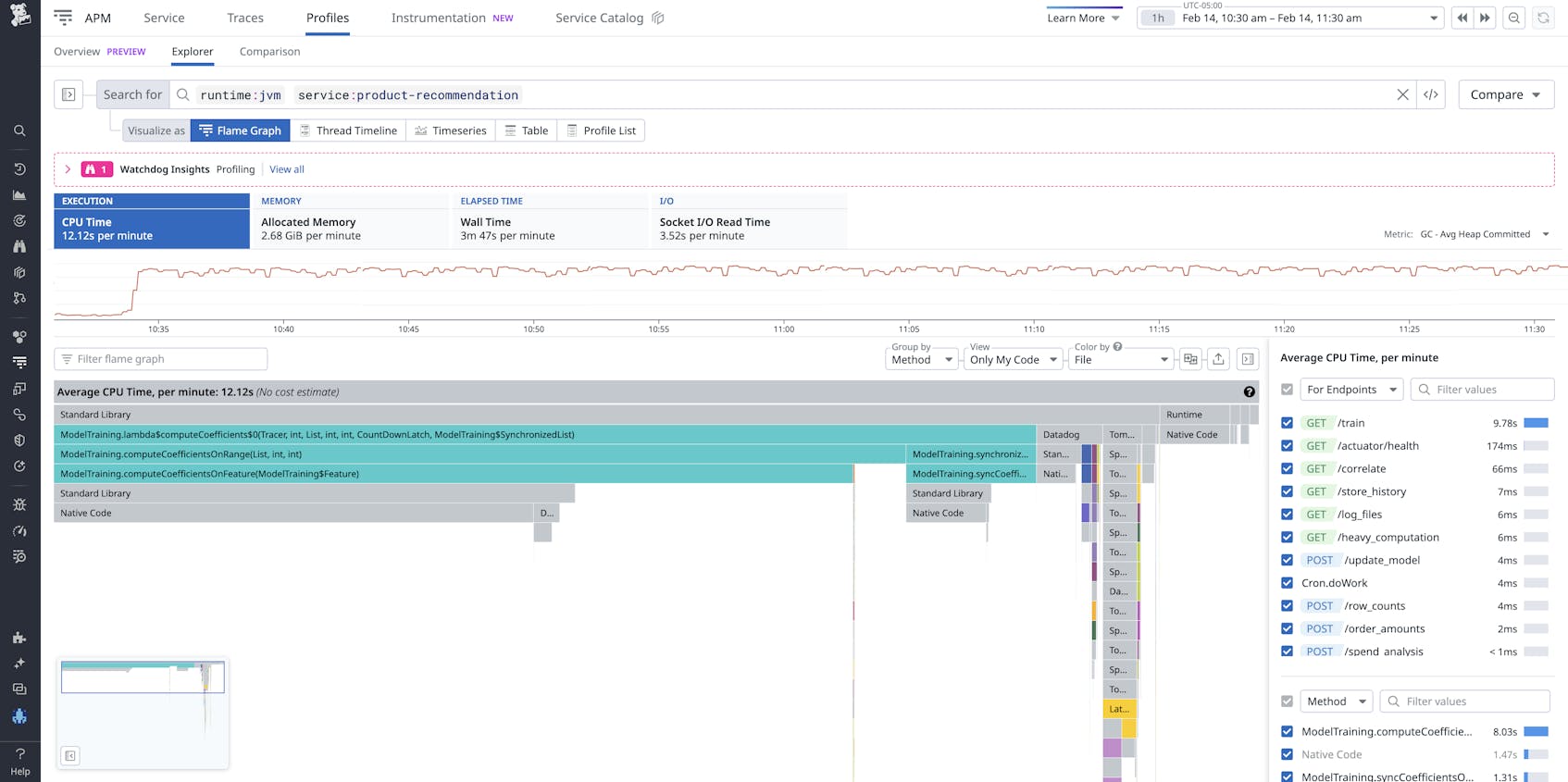
To illustrate how this works, let’s say you have a Java-based e-commerce application deployed on a Kubernetes cluster. The application runs a Quarkus service that handles API requests. While monitoring the application in Datadog profiling, you notice a spike in CPU usage for the /product-recommendation endpoint, which appears related to a model-training database query.
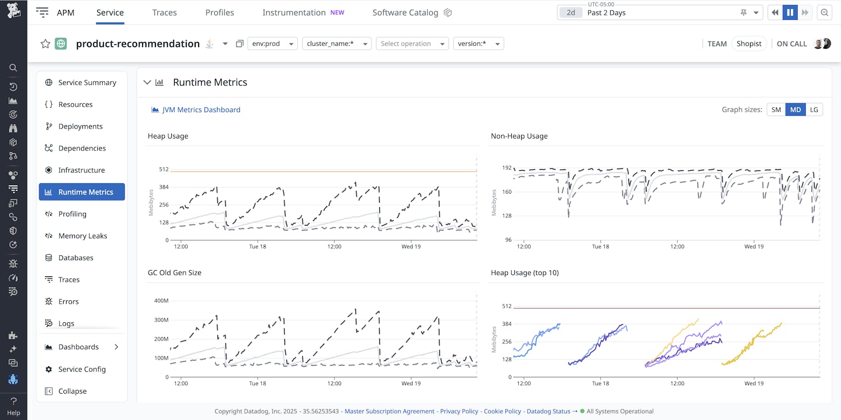
You switch over to the Runtime Metrics view in the service dashboard to see if the application is under pressure. You find that heap memory usage and GC size are repeatedly spiking and then mysteriously dropping to zero.
Confused by the periodic nature of the heap usage graph, you then pivot to Kubernetes container monitoring to investigate the pod hosting the application. The memory usage graphs here match the memory usage patterns. It looks like the container is regularly getting killed and relaunched.
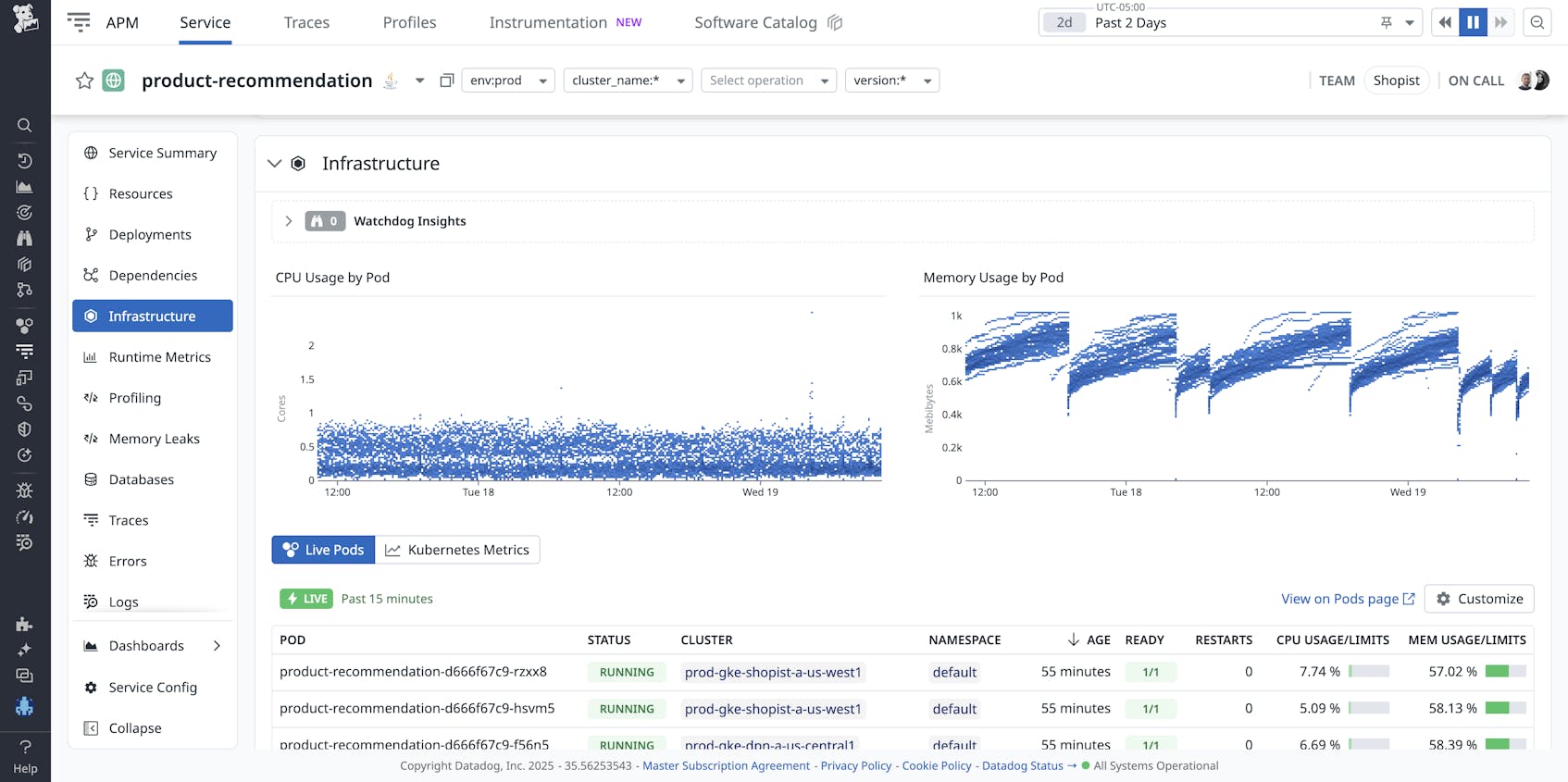
Inspecting the pod’s history confirms that the container is regularly getting OOM killed.
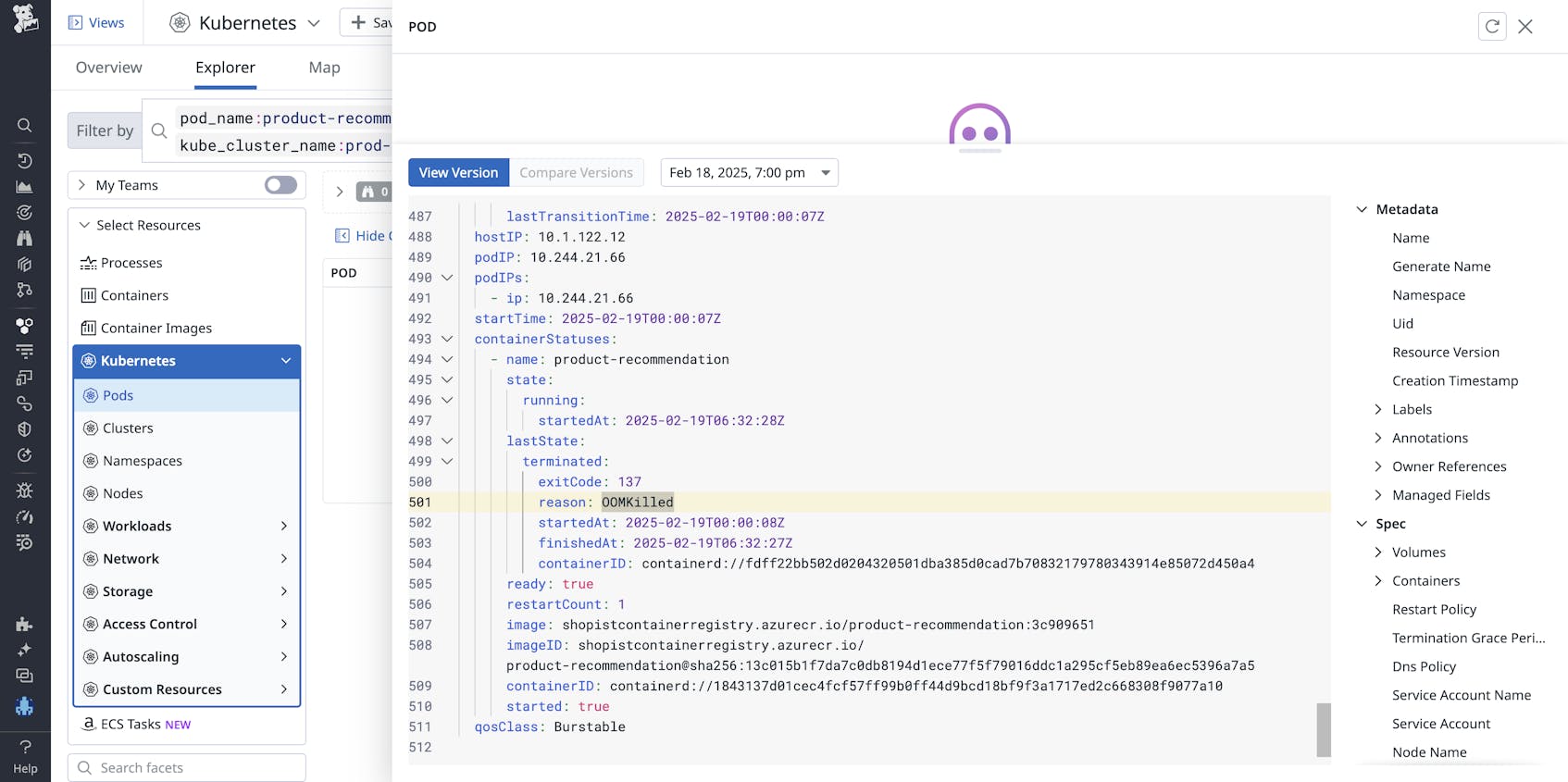
You try increasing the memory limits of the pod to stop the OOM kills. If the issue is simply GC pressure, ascribing more memory to the workload should resolve it. However, due to the linear growth of the heap, you also suspect that the native code may be leaking—so you push a ticket to the developer’s backlog to investigate.
More to come
In a future blog post, we'll show you more in-depth profiling-based optimization strategies and how we've implemented them on a large scale at Datadog.
Optimize Java application performance on Kubernetes
In this post, we’ve explored the JVM and showed how proper tuning can make your Java applications run faster and more efficiently in Kubernetes environments. We’ve also offered an example of how you can monitor these applications in Datadog to help ensure consistently high performance.
If you’re interested in learning more, check out our other blog posts on monitoring Java runtime, Java memory management, or Datadog’s Continuous Profiler. If you’re new to Datadog and would like to monitor the health and performance of your Java applications on Kubernetes, sign up for a free trial to get started.
