
Datadog collects billions of events from millions of hosts every minute and that number keeps growing and fast. Our data volumes grew 30x between 2017 and 2022. On top of that, the kind of queries we receive from our users has changed significantly. Why? Because our customers have grown in sophistication: they run more complex stacks, want to monitor more data, and run more complex analyses. That, in turn, puts pressure on our timeseries data store.
Data stores have a number of tricks in their bag to offer good performance. One of the most critical ones is the judicious use of indices, a key data structure that can make queries fast and efficient, or unbearably slow. Over the years, our homegrown indices that were put in place in 2016 became a performance bottleneck for queries and a source of increased maintenance. We knew that we had to learn from these challenges and come up with something better.
This blog post provides an overview of the Datadog timeseries database and the challenges of timeseries indexing at scale. We’ll compare the performance and reliability of two generations of indexing services.
Metrics platform overview
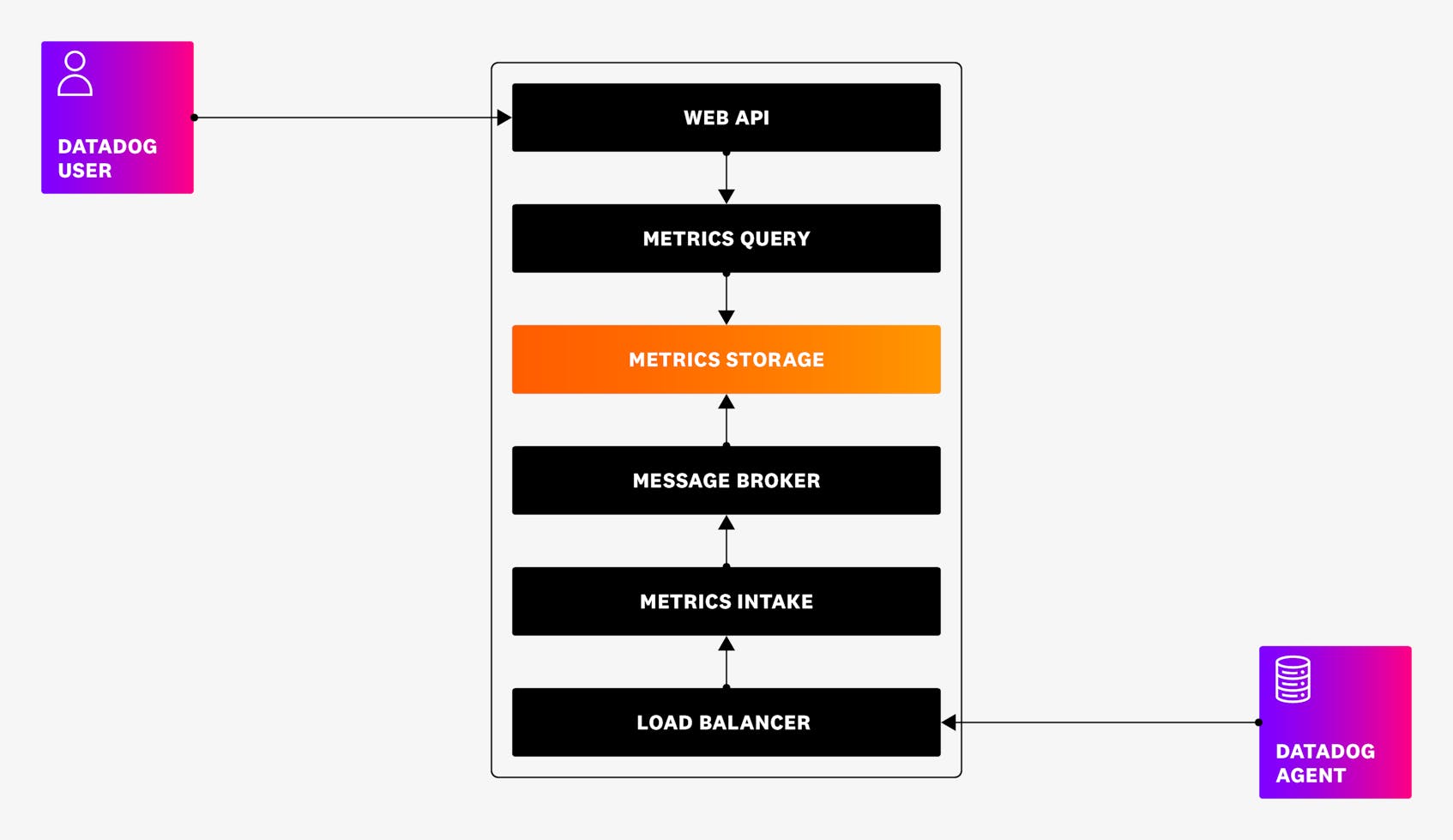
From a high level, the metrics platform consists of three major components: intake, storage, and query. As shown in the image below, the Datadog Agent receives data and sends it to the load balancer. The data then gets ingested by metrics intake and written to the message broker. The metrics storage component then reads the data from the message broker and stores it on a disk in the timeseries database. When a Datadog user sends a query (see the example below), the query is sent to the API gateway and gets executed by the metrics query engine.
Intake
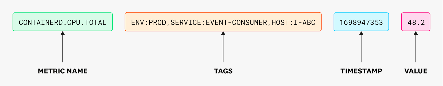
Metrics intake is responsible for ingesting a stream of data points that consist of a metric name, zero or more tags, a timestamp, and a value. Tags are a way of adding dimensions to Datadog metrics so they can be filtered, aggregated, and compared. A tag can be in the format of value or key:value. Commonly used tag keys are env, host, and service. Additionally, Datadog allows users to submit custom tags. The timestamp records the time when the data point was generated. Finally, the value is a numerical value that can track anything about the monitored environment, from CPU usage and error rates to the number of user sign-ups.
This is what a typical ingested data point looks like:
The ingested points are processed and written into Kafka, a durable message broker. Kafka allows multiple services and teams to consume the same data stream independently and for different purposes, such as analysis, indexing, and archiving for long-term storage.
Storage
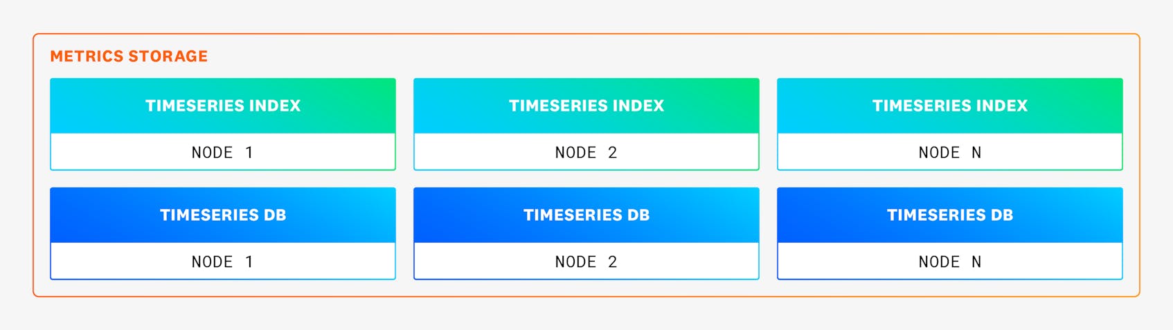
One of these Kafka consumers is the short-term metrics storage layer, which is split into two individually deployed services. The first one is the Timeseries Database service, which stores the timeseries identifiers, timestamps, and values as tuples of <timeseries_id, timestamp, float64>. The second service is responsible for indexing the identifiers and tags associated with them and stores them as tuples of <timeseries_id, tags>. This is the Timeseries Index service, which is a custom database built on top of RocksDB and is responsible for filtering and grouping timeseries points during query execution.
Query
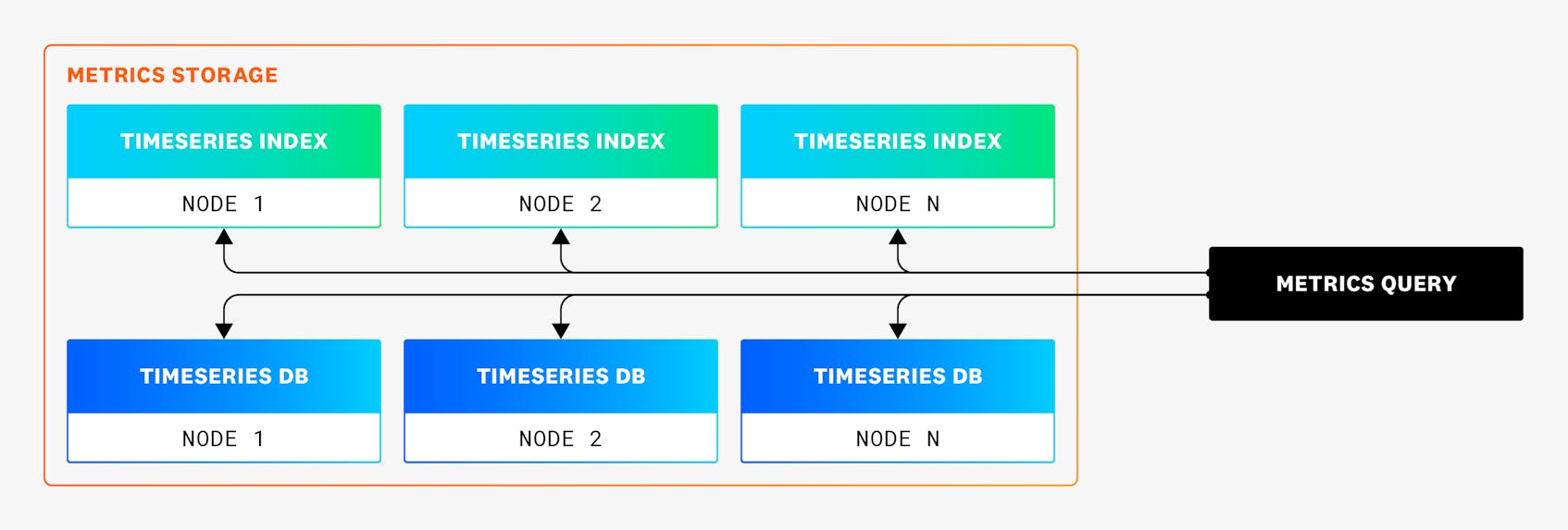
The distributed query layer connects to the individual timeseries index nodes, fetches intermediate query results from the timeseries database, and combines them.
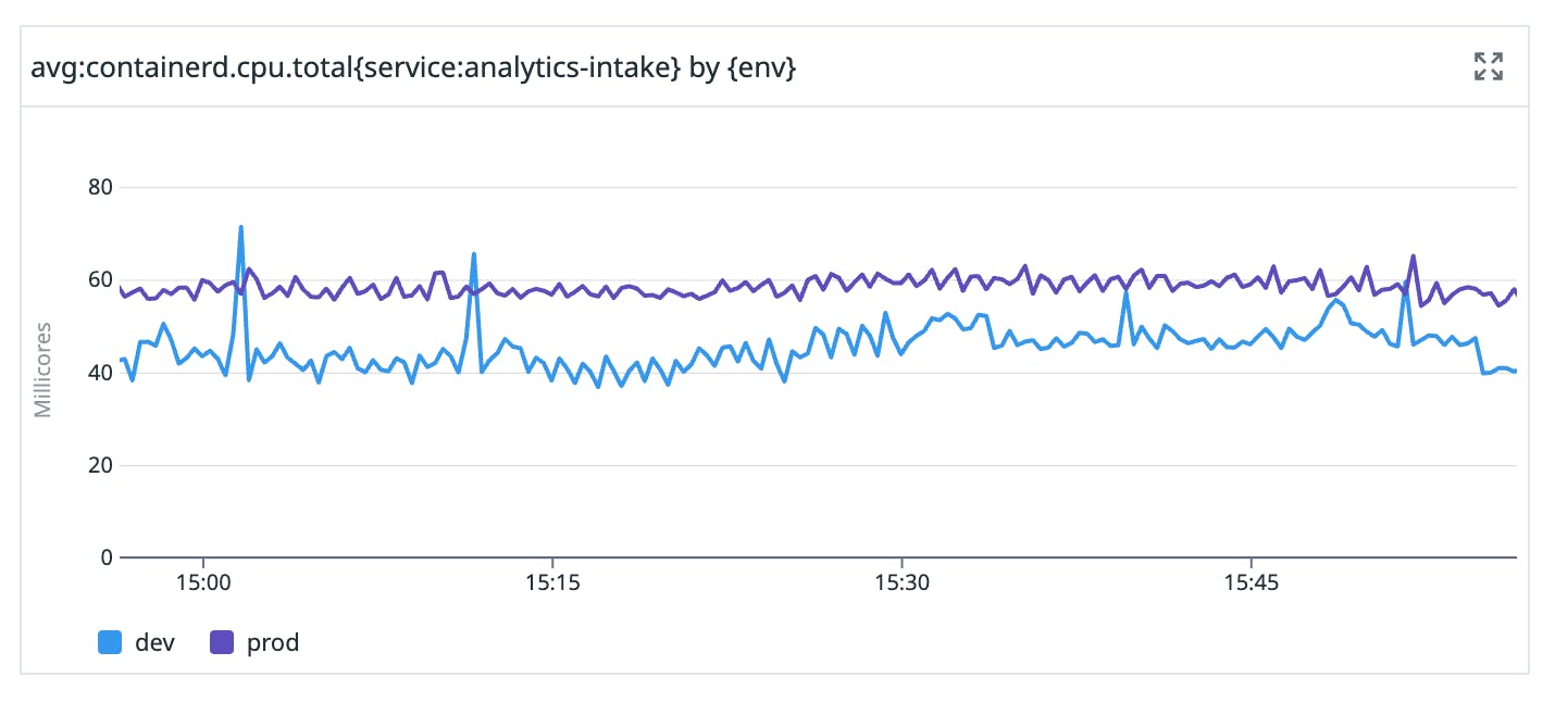
This is what a typical query looks like:
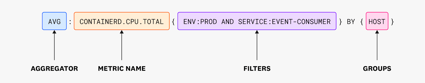
Filters are used to narrow down a queried metric to a specific subset of data points, based on their tags. They are particularly useful when the same metric is submitted by many hosts and services, but you need to look at a specific one. In this particular example, the env:prod AND service:event-consumer filter tells the query engine to include only data points that come from the service called event-consumer that is running in the production environment.
The groups, which are also based on tags, drive the query results. The grouping process produces a single timeseries, or a single line in a line graph, for each unique group. For example, if you have hundreds of hosts spread across four services, grouping by service allows you to graph one line for each service.
The data points within each group are then combined according to the aggregator function. In the following example, the avg aggregator computes an average value across all hosts for a specific service, grouped by environment:
Original indexing service
Now that you know where the timeseries database fits into the architecture, let’s get back to indexing. We index timeseries points by their tags to make query execution more efficient and avoid scanning the data for the entire metric when only a small subset is requested. Scanning the data for the entire metric would be similar to a full table scan in SQL databases.
Datadog’s original indexing strategy relied heavily on automatically generating indexes based on the query log of a live system. Every time the system encountered a slow or resource-consuming query, it would record the information about the received query in a log that was periodically analyzed by a background process. The process looked at the number of queries, the query execution time, the number of input (scanned) timeseries identifiers, and the number of output (returned) identifiers. Based on these parameters, the process would then find and create indexes for highly selective queries, meaning queries with high input-to-output ratios.
Additionally, the indexes that became obsolete and stopped receiving queries would get removed from the system. Automatically generated indexes were highly effective in reducing the amount of CPU and memory resources spent on repetitive queries. The indexes would create materialized views of resource-consuming queries, turning a slow full table scan into a single key-value lookup.
Design
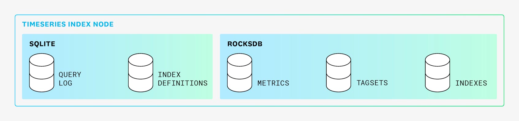
The original timeseries index service was implemented in Go with the help of embedded data stores: SQLite and RocksDB. Embedded means these data stores are not running on a separate server or a standalone process, and instead are integrated directly into an application. We used SQLite, the most widely deployed SQL engine, to store metadata such as the index definitions and the query log:
CREATE TABLE index_definitions (
	metric_name TEXT,
	filter_tags TEXT,
	query_count INTEGER,	-- number of times the index was queried
	timestamp INTEGER,
	PRIMARY KEY (metric, filters)
);

CREATE TABLE query_log (
	metric_name TEXT,
	filter_tags TEXT,
	inputs INTEGER,		-- number of input (scanned) ids
	outputs INTEGER,	-- number of output (returned) ids
	duration_msec INTEGER,
	timestamp INTEGER,
	PRIMARY KEY (query_id)
);
The index definition table was read-heavy, updated infrequently and cached entirely in memory. The query log was bulk updated in the background outside of the ingest and query paths. The flexibility of SQL was convenient for debugging because we could easily inspect and modify the tables using the sqlite3 CLI.
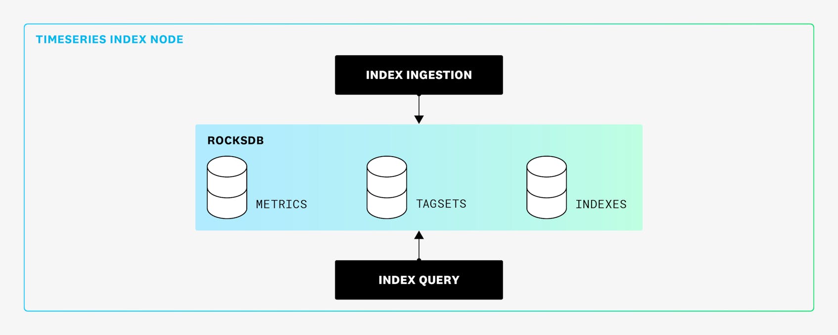
The heavy-lifting was the handling of all writes, required for indexing trillions of events per day, and done using RocksDB. RocksDB is a key-value store that powers production databases and indexing services at big tech companies such as Meta, Microsoft, and Netflix. The Datadog timeseries index service maintained three RocksDB databases per node: Tagsets, Metrics, and Indexes.
The Tagsets database stored a mapping of timeseries IDs to tags associated with them. The key was the timeseries ID and the value was the set of tags. If you consider these six data points:
| Metric Name | Timeseries ID | Tags |
|---|---|---|
| cpu.total | 1 | env:prod,service:web,host:i-187 |
| cpu.total | 2 | env:prod,service:web,host:i-223 |
| cpu.total | 3 | env:staging,service:web,host:i-398 |
| cpu.total | 7 | env:prod,service:db,host:i-409 |
| cpu.total | 8 | env:prod,service:db,host:i-543 |
| cpu.total | 9 | env:staging,service:db,host:i-681 |
This is how the data was stored in the Tagsets database:
| Key (timeseries ID) | Value (tags) |
|---|---|
| 1 | env:prod,service:web,host:i-187 |
| 2 | env:prod,service:web,host:i-223 |
| 3 | env:staging,service:web,host:i-398 |
| 7 | env:prod,service:db,host:i-409 |
| 8 | env:prod,service:db,host:i-543 |
| 9 | env:staging,service:db,host:i-681 |
And the Metrics database contained a list of timeseries IDs per metric:
| Key (metric) | Value (timeseries ID) |
|---|---|
| cpu.total | 1,2,3,7,8,9 |
The Tagsets and Metrics databases alone were enough to run queries. Consider the query cpu.total{service:web AND host:i-187}. To execute it, first you need to get all the timeseries IDs for the metric cpu.total from the Metrics database. This then translates into a single RocksDB key-value lookup for the key cpu.total, which returns the values: 1,2,3,7,8,9.
After we get all the timeseries IDs, we query each ID from the Tagsets database to check whether the associated tags matched the filters. The approach was similar to full table scans in SQL databases where we had to look at all possible tag sets for the metric. Its main downside was that the number of Tagsets lookups grew linearly with the number of timeseries per metric, which in some cases was a challenge for high cardinality metrics. In this particular example, we needed to look up seven keys in total; one key from the Metrics database and six keys from the Tagsets database, one key for each timeseries ID.
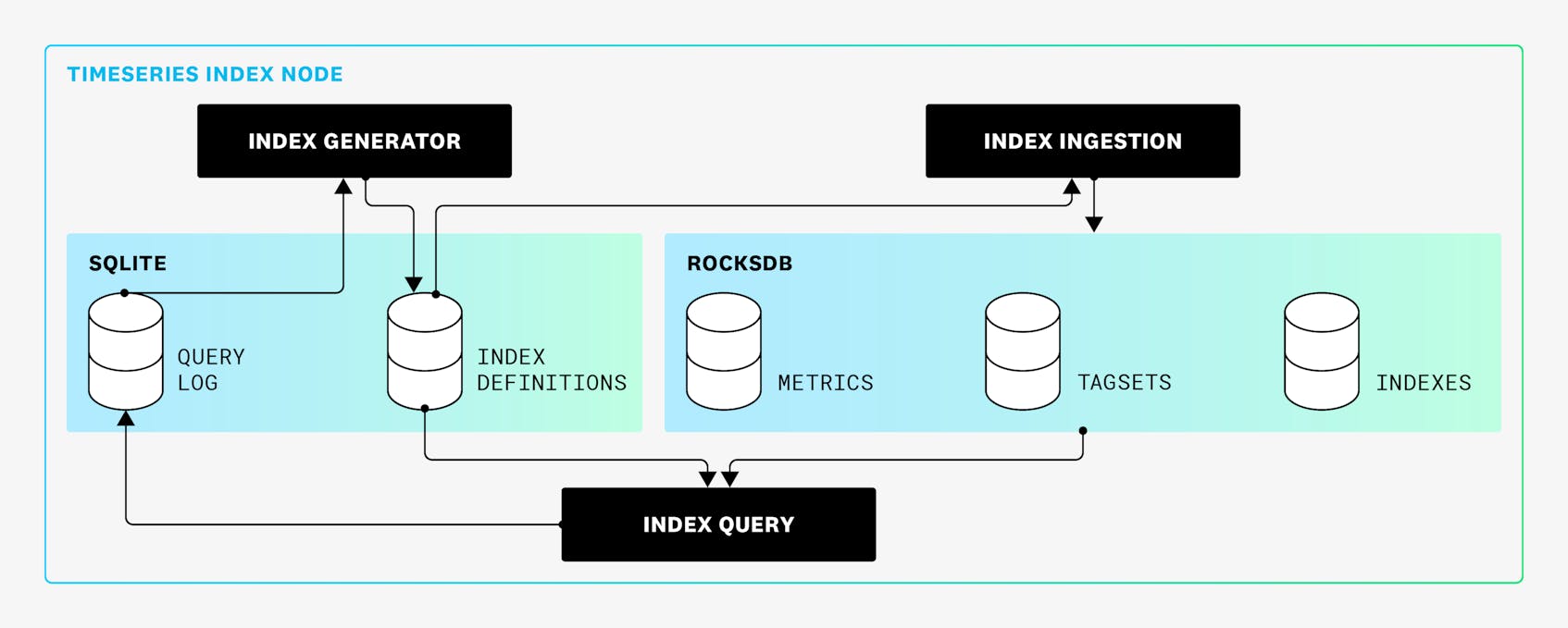
To avoid full scans, resource-consuming queries were indexed in the Indexes RocksDB database. Every resource-consuming query was logged in the query_log SQLite table. Periodically, a background process queried the table and would create a new index in the index_definitions table for those resource-consuming queries. The ingestion path checked whether the ingested timeseries belonged to an index, and if it did, the ID would be written to the Indexes database in addition to the Tagsets and Metrics databases.
This is how the Indexes database would look like if we created two indexes for the metric cpu.total; one index for the service:web,host:i-187 filters and another for the service:db filter.
| Key (metric;tags) | Value (timeseries IDs) |
|---|---|
| cpu.total;service:web,host:i-187 | 1 |
| cpu.total;service:db | 7,8,9 |
Now, if someone queries cpu.total{service:web AND host:i-187}, the query planner tries to match the metric and the filters against the index definitions. Because there was an index for the exact filters the query was asking for (the tags service:web and host:i-187), the query would get its results directly from the Indexes database, without having to access the Tagsets and Metrics databases. The query that previously required scanning Tagsets and making seven RocksDB lookups, now only needed a single lookup.
Advantages
For Datadog Metrics, like most monitoring systems, the ratio of queried-to-written timeseries data points is typically low. On average, we see roughly only 30% of the written data being consistently queried, making this indexing strategy space efficient. We had to cover only a subset of the ingested data with indexes to make most queries perform well.
Challenges
Automatically generated indexes worked well for programmatic query sources such as periodic jobs or alerting. However, user-facing queries are less predictable, and they often fell back to full table scans, leading to query timeouts and poor user experiences. Additionally, even programmatic query sources occasionally change their query patterns significantly, making the existing indexes inefficient and overloading the database with many new resource-consuming queries. It wasn’t uncommon for such incidents to require manual intervention where an engineer would remove or create indexes by hand.
Next-gen indexing service
The manual operational toil was growing and the metrics queries were slowly getting less performant. It was time to rethink how we index timeseries data at Datadog. The new indexing strategy we came up with was inspired by the core data structure behind search engines, the inverted index. In search engines, the inverted index associates every word in a document with document identifiers that contain the word.
For example:
documents = {
    1: "a donut on a glass plate",
    2: "only the donut",
    3: "listen to the drum machine",
}

index = {
    "a": [1],
    "donut": [1, 2],
    "on": [1],
    "glass": [1],
    "plate": [1],
    "only": [2],
    "the": [2, 3],
    "listen": [3],
    "to": [3],
    "drum": [3],
    "machine": [3],
}
A real-world example of the inverted index is an index in a book where a term references a page number:
Taking the definition of an inverted index for search engines, if we replace the term “document identifier” with “timeseries identifier” and “word” with “tag,” we have a definition for an inverted index for timeseries data. The inverted index associates every tag in a timeseries with the identifiers of timeseries that contain the tag.
Design
The new design required rewriting almost the entire timeseries index service. It gave us an opportunity to reevaluate the tech stack we used. The new approach didn’t require maintaining any metadata, so that removed the SQLite dependency. RocksDB for the original implementation was a solid choice—we didn’t have any issues with it in production—so we kept it as the key-value store for indexes.
We’ll use the same six data points from the previous example to see how the next-gen strategy works. The Tagsets and Metrics databases look almost the same as in the original implementation so we won’t go over them again. The major difference between the original and next-gen implementation is the Indexes database, where we now unconditionally index every ingested tag, similarly to what search engines do with the inverted index:
| Key (metric;tag) | Value (timeseries IDs) |
|---|---|
| cpu.total;env:prod | 1,2,7,8 |
| cpu.total;env:staging | 2,9 |
| cpu.total;service:web | 1,2,3 |
| cpu.total;service:db | 7,8,9 |
| cpu.total;host:i-187 | 1 |
| cpu.total;host:i-223 | 2 |
| cpu.total;host:i-398 | 3 |
| cpu.total;host:i-409 | 7 |
| cpu.total;host:i-543 | 8 |
| cpu.total;host:i-681 | 9 |
The timeseries queries map well to the inverted index. To execute a query, the query engine makes a single key-value lookup for each queried tag and retrieves a set of relevant timeseries identifiers. Then, depending on the query, the sets are combined either by computing a set intersection or a set union.
For example, for the query cpu.total{service:web AND host:i-187}, we do two key-value lookups from the Indexes databases. The first is to retrieve the cpu.total;service:web key, which returns the values: 1,2,3. The second key-value lookup is for the key cpu.total;host:i-187, which returns the value: 1.
To get the final result, we compute the set intersection between the two returned values, 1,2,3 and 1, which is 1. For the same query, the previous indexing strategy required a single lookup when the index existed, and seven lookups when there was no index. With the new indexing strategy we get a consistent query performance because the query always requires exactly two lookups.
Challenges
One downside of this strategy is the write and space amplification. Every unique timeseries identifier has to be stored multiple times, once for each tag. With tens of tags per single timeseries, we have to store each timeseries identifier more than 10 times. Our early tests confirmed the concern that the timeseries index had to write and store noticeably more data on the disk. However, previously the timeseries index barely utilized the disk and was strictly CPU bound, so the disk space utilization wouldn’t become a problem even if we had to start storing an order of magnitude more data.
The write amplification and the increased CPU utilization the new strategy could bring was still a concern. However, it turned out not to be an issue, as we will see.
Advantages
The new timeseries index doesn’t rely on the query log or a list of automatically generated indexes. It simplifies the ingestion path and makes it less CPU-intensive because it doesn’t have to match every ingested timeseries against the list of indexes to find which index it belongs to. Same is true for queries: we no longer need to do any index matching because we know that an index for every tag always exists. It also removes the need for running several CPU-consuming background jobs responsible for maintaining the indexes. The timeseries index doesn’t have to scan the query log anymore and we never need to backfill newly created indexes. Overall, while we have to write more data, we now spend less CPU time doing it.
On the query side, on average, indexed queries become slightly more expensive because some queries, which previously required a single key-value lookup, now require multiple lookups. On the other hand, every possible query now always has a partial index available. Since we don’t have to ever fall back to a full table scan, the worst case scenario for query performance improved and became more predictable.
Intranode Sharding
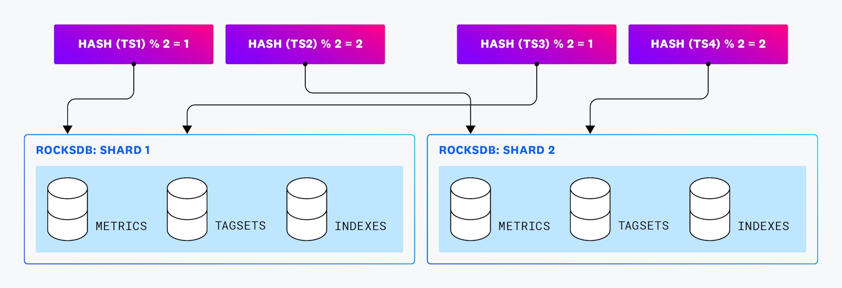
Another performance issue with the original implementation was that the query path didn’t scale with CPU cores available on a node. No matter how many CPU cores a node had, a single query couldn’t use more than a single core. At some point, the single-core performance would always become a bottleneck for how quickly the service could execute a query. One of the goals of designing the new service was being able to scale ingest and queries with CPU cores. We accomplished this by making each node split RocksDB indexes into multiple isolated instances (shards), each responsible for a subset of timeseries. To ensure the data is distributed evenly across the shards, we hash the ingested timeseries IDs and assign a timeseries to a particular shard based on the hash.
To execute a single query, the service fetches data from each RocksDB shard in parallel and then merges the results.
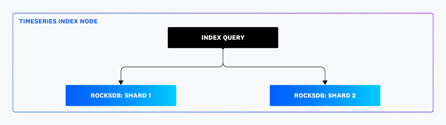
After running experiments in production, we settled on creating eight shards on a node with 32 CPU cores. It gave us a nearly 8x performance boost without adding too much overhead from splitting and having to merge the timeseries back. Additionally, the intranode sharding allowed us to switch to larger cloud node types with more CPU cores, reducing the total number of nodes we had to run.
Switching to Rust
While the Go language worked well for most services at Datadog, it wasn’t the best fit for our resource-intensive use case. The service spent nearly 30% of CPU resources on garbage collection, and we reached the point where implementing performance optimizations was very time consuming. We needed a compiled language with no garbage collector. We decided to give Rust a chance, which turned out to be the right choice. To illustrate the performance differences, we’ll compare Go and Rust on two CPU-demanding operations that the indexing service executes.
When grouping timeseries, the service needs to extract tags for relevant tag keys. For example, grouping env:prod,service:web,host:i-187 by env and host is expected to produce a group env:prod,host:i-187. Here is a simplified version of what we run in production:
fn has_group(tag: &str, group: &str) -> bool {
    tag.len() > group.len() && tag.as_bytes()[group.len()] == b':' && tag.starts_with(group)
}

fn group_key(tags: &[&str], groups: &[&str]) -> String {
    let mut key_tags = Vec::with_capacity(groups.len());
    for tag in tags {
        for group in groups {
            if has_group(tag, group) {
                key_tags.push(*tag);
            }
        }
    }
    key_tags.sort_unstable();
    key_tags.dedup();
    key_tags.join(",")
}
And here is a one-to-one translation to Go:
func hasKey(s string, group string) bool {
	return len(s) > len(group) && s[len(group)] == ':' && strings.HasPrefix(s, group)
}

func groupKey(tags []string, groups []string) string {
	keyTags := make([]string, 0, len(groups))
	for _, tag := range tags {
		for _, group := range groups {
			if hasKey(tag, group) {
				keyTags = append(keyTags, tag)
			}
		}
	}
	sort.Strings(keyTags)
	keyTags = slices.Compact(keyTags)
	return strings.Join(keyTags, ",")
}
While the functions look very similar, our benchmarks on production data on an AWS c7i.xlarge instance (Intel Xeon Platinum 8488C) showed that the Rust version is three times faster than the Go version.
As a part of the ingest and the query paths, the indexing service needs to merge many timeseries IDs together. The IDs are integers, stored as sorted arrays. For example, merging three arrays of IDs [3,6], [4,5], [1,2] is expected to produce a single sorted array containing a union of all IDs: [1,2,3,4,5,6]. The problem can be solved with the k-way merge algorithm using a min-heap. Luckily, the Rust and the Go standard libraries come with a heap implementation we can use to implement this. Let’s start with the Rust version, as the implementation is slightly more straightforward:
#[derive(Eq)]
struct Item<'a> {
    first: u64,
    remainder: &'a [u64],
}

impl Ord for Item<'_> {
    fn cmp(&self, other: &Self) -> Ordering {
        other.first.cmp(&self.first)
    }
}
impl PartialOrd for Item<'_> {
    fn partial_cmp(&self, other: &Self) -> Option<Ordering> {
        Some(self.cmp(other))
    }
}
impl PartialEq for Item<'_> {
    fn eq(&self, other: &Self) -> bool {
        self.first == other.first
    }
}

fn merge_u64s(sets: &[Vec<u64>]) -> Vec<u64> {
    let mut heap = sets
        .iter()
        .map(|set| Item {
            first: set[0],
            remainder: &set[1..],
        })
        .collect::<BinaryHeap<Item>>();
    let mut result = Vec::new();
    // Use peek_mut instead of pop + push to avoid sifting the heap twice.
    while let Some(mut item) = heap.peek_mut() {
        let Item { first, remainder } = &*item;
        if result.last() != Some(first) {
            result.push(*first);
        }
        if !remainder.is_empty() {
            *item = Item {
                first: remainder[0],
                remainder: &remainder[1..],
            };
        } else {
            PeekMut::pop(item);
        }
    }
    result
}
Merging 100 sets of 10K integers in Rust using the code above takes 33ms.
And here is the Go version:
type Item struct {
	first     uint64
	remainder []uint64
}

type Uint64SetHeap []Item
func (h Uint64SetHeap) Len() int           { return len(h) }
func (h Uint64SetHeap) Less(i, j int) bool { return h[i].first < h[j].first }
func (h Uint64SetHeap) Swap(i, j int)      { h[i], h[j] = h[j], h[i] }

func mergeUint64s(sets [][]uint64) []uint64 {
	h := make(Uint64SetHeap, 0, len(sets))
	for _, set := range sets {
		h = append(h, Item{first: set[0], remainder: set[1:]})
	}
	heap.Init(&h)
	var result []uint64
	for h.Len() > 0 {
		item := h[0]
		if len(result) == 0 || result[len(result)-1] != item.first {
			result = append(result, item.first)
		}
		if len(item.remainder) > 0 {
			h[0] = Item{first: item.remainder[0], remainder: item.remainder[1:]}
		} else {
			// No more elements in the set, remove the set from the heap.
			n := len(h) - 1
			h[0] = h[n]
			h = h[:n]
		}
		// The value of the head changed. Re-establish the heap ordering.
		heap.Fix(&h, 0)
	}
	return result
}
We see a similar result again: in Go, merging the same 100 sets, 10K integers each, takes three times longer—101ms. To make this benchmark more fair, however, there is one optimization we can do in Go. If we look closer at the heap implementation in Rust, we notice that the BinaryHeap structure in Rust is generic, meaning the generic type T is replaced with our concrete type Item during compilation. The Go heap implementation does not use generics: instead, it uses the heap.Interface interface. Interfaces in Go come with an additional cost in runtime and make some optimizations, such as inlining, impossible. Go supports generics since version 1.18, but unfortunately there is no generic heap in the standard library yet (see the GitHub issue discussing adding it). Instead of trying to write a generic heap in Go, we can do what the Rust compiler does for us by hand: copy the container/heap package and manually replace all instances of heap.Interface with Item. There is a lot of code to copy and paste, so I won’t include it here. This new version is faster—it takes 76ms to run, but is still more than twice as slow as the Rust version.
These are not isolated cases, we found several other CPU-demanding operations being faster in Rust. We learned that while in many cases it’s possible to make Go as fast as Rust, writing performance-sensitive code in Go requires a relatively larger time investment and deeper language expertise.
Conclusion
To summarize the changes we made, we adapted an entirely different indexing strategy: we now always index the timeseries to avoid full scans. We sharded the indexing nodes internally to parallelize query execution and take advantage of larger nodes with more CPU cores. Finally, we rewrote the service from Go to Rust, making CPU-demanding operations up to 6x faster. Combined, these changes allowed us to query 20 times higher cardinality metrics on the same hardware, and we significantly reduced the tail query latency. This resulted in a 99% reduction of query timeouts and made the timeseries index nearly 50% cheaper to run.
Excited about high-performance Rust? Datadog is hiring. Stay tuned for more blog posts on timeseries databases and Rust!